Pipeline Modules
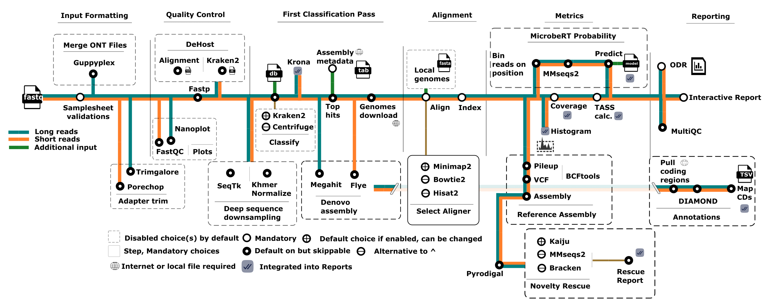
This page describes each step in the TaxTriage workflow in execution order - what it does, which tool is used, and what it produces.
Step −1: SRA / ENA Retrieval (Optional)
Modules: SRA_RESOLVE, SRA_FETCH_ENA, SRA_FETCH_SRATOOLS Trigger: any fastq_1 value (samplesheet column or --fastq_1) that is an accession rather than a path
Runs before everything else, only when accessions are present.
SRA_RESOLVEbatches every accession into one lookup against the ENA Portal API (falling back to NCBI eutils), expanding experiment/sample/project accessions into their child runs and recording each run's FASTQ URLs, md5s, instrument platform and paired-end layout.SRA_FETCH_ENAdownloads ENA's pre-splitfastq.gzfiles and verifies them against the published md5.SRA_FETCH_SRATOOLShandles runs ENA does not host, viaprefetch+fasterq-dump --split-3.
Downloaded reads enter the pipeline as ordinary samples, so every step below is unchanged. Files are cached under <outdir>/sra_downloads/ (or --sra_cache_dir) and reused on later runs instead of being downloaded again.
See Samplesheet → SRA / ENA Accessions.
Step 0: Pre-Aligned Input Preparation (Optional)
Modules: PREPARE_BAM, BAM_CONSENSUS Trigger: any bam value (samplesheet column or --bam)
Runs in place of read processing, only for samples that arrive pre-aligned.
PREPARE_BAMnormalises the container to BAM (CRAM is decoded, SAM is compressed, BAM is left alone), coordinate-sorts it unless the@HD SO:header already says it is sorted, writes a.csiindex, and emits a primary-read count.--bam_minmapqapplies asamtools view -qfilter here if you asked for one.BAM_CONSENSUSruns only when no--reference_fastawas supplied, callingsamtools consensus -aoff the alignment so sourmash sketching, the shared-window conflict report and the ANI matrix have bases to work with. References whose consensus is almost entirelyNare dropped.
The resulting [meta, bam, csi] tuple has the same shape as the aligner's own output, so everything downstream is unchanged. A recovered consensus FASTA is fuzzy-matched against the assembly summary exactly like a user-supplied reference, producing the accession → taxid map match_paths.py needs.
Pre-aligned samples skip Steps 1 through 5 entirely and are excluded from reference download.
See Pre-Aligned Input.
Step 0: Subsampling (Optional)
Tool: Khmer Normalization or Seqtk Parameter: --downsample (Khmer) or --subsample <N> (Seqtk)
Reduces each sample to N reads before any downstream processing. Useful for a fast "triage" analysis when input datasets are very large.
Step 1: Quality Control - Part 1
Illumina
Tool: FastQC
Parameter: --skip_plots to disable
Generates quality score distributions, adapter content plots, and per-base quality reports. These are the default read-QC plots in the MultiQC report (fastp is off by default, see Step 2b).
Oxford Nanopore
Tool: pycoQC (requires --sequencing_summary) for Illumina, NanoPlot for ONT
Generates read length/quality plots from raw ONT output. NanoPlot is run on the raw reads. pycoQC uses the sequencing summary file for additional detail.
Step 2: Adapter Trimming
Illumina
Tool: Trimgalore
Parameter: samplesheet trim column (--trim for --fastq_1 runs); --skip_trimming turns it off for all samples
Removes adapter sequences from paired or single-end Illumina reads.
Oxford Nanopore
Tool: Porechop
Parameter: samplesheet trim column (--trim for --fastq_1 runs); --skip_trimming turns it off for all samples
Removes adapter sequences from ONT reads.
Step 2b: Quality Filtering with fastp / fastplong (Optional, off by default)
Tool: fastp (Illumina), fastplong (ONT / PacBio)
Parameters: --enable_fastp, --minq <N> (fastplong minimum quality, default 7)
fastp is disabled by default. Pass --enable_fastp to run it after adapter trimming and before classification. A sample fastp cannot process keeps its unfiltered reads instead of dropping out of the run.
Without --enable_fastp (default) | With --enable_fastp | |
|---|---|---|
| Reads passed to classification | Trimmed (samples with trim=TRUE) or raw reads | fastp / fastplong-filtered reads |
--minq | Ignored | Applied by fastplong |
| Output folders | none | fastp/, fastplong/ |
| MultiQC read QC | FastQC / NanoPlot, plus Trim Galore (cutadapt) stats for samples with trim=TRUE | Same, plus the fastp section |
--skip_fastphas been removed. It is no longer needed because fastp is off unless requested; passing it only prints a warning.
Step 3: Host Removal (Optional)
Tool: Minimap2 or Kraken2 (with --filter_kraken2) Parameters: --genome, --remove_reference_file, --min_mapq_host, --filter_kraken2 <k2_db>
Reads that align to the host reference (e.g., human genome) are removed. Unclassified (non-host) reads are retained for classification.
Studies show Minimap2 has a slightly lower false-negative rate than Bowtie2 for host depletion. See PMC9040843 and s41467-021-26865-w.
Step 4: Metagenomics Classification
Tool: Kraken2 (default) or Centrifuge
Parameters: --db, --k2_confidence, --skip_kraken2, --centrifuge
Each read is classified against the Kraken2 (or Centrifuge) database. Results are summarized in a Kraken2 report and visualized as interactive Krona plots - the most important early output for understanding abundance from a metagenomics perspective.
⚠️ Always consider the limitations of your database. Organisms absent from the database cannot be classified. See available databases.
Step 5: Top Hits Assignment
Parameters: --top_hits_count, --top_per_taxa, --pathogens, --add_irregular_top_hits
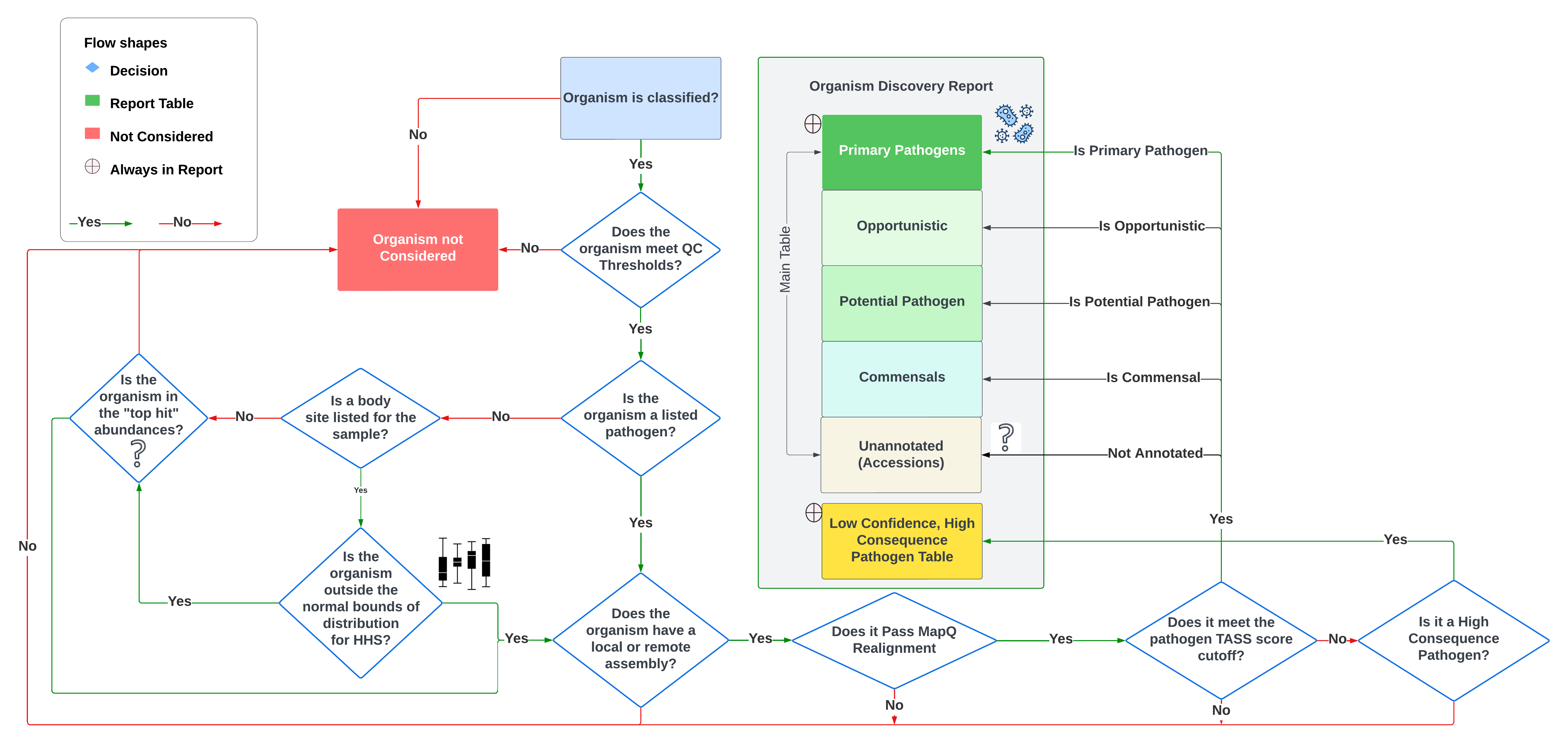
Not all classified organisms are aligned - only "top hits" proceed to alignment. The selection follows this decision tree:
Top hits include:
- Any organism annotated in the pathogen sheet (regardless of abundance)
- The top N organisms per taxonomic rank (controlled by
--top_hits_countand--top_per_taxa) - Organisms with irregular HMP abundance distributions (if
--add_irregular_top_hitsis set)
Step 6: Reference Preparation
Parameters: --assembly, --reference_fasta, --organisms
Reference genomes for all top hit organisms are obtained:
- Default (internet): Downloaded from NCBI FTP using the assembly summary file.
- Offline: Provided via
--reference_fasta(local FASTA) or--assembly(local assembly summary).
Which assembly is chosen per organism follows the Assembly Selection Order: a curated assembly_accession from the pathogen sheet is used first (accession-first), otherwise the best local taxid match is picked by priority tier (representative → reference → complete genome → other), preferring RefSeq over GenBank on ties.
A FASTA index is built for Bowtie2 (Illumina) at this stage.
Step 7: Alignment
Illumina
Tool: Minimap2 (default), Hisat2, Bowtie2 (with --use_bt2)
ONT / PacBio
Tool: Minimap2
All Kraken2-classified reads (or all raw reads if --skip_kraken2) are aligned to the reference genomes. Only the best-scoring alignment per read is currently retained.
Note: Minimap2 is used for both data types in the host removal step, but BWA-MEM2/Bowtie2 is used for Illumina in the classification alignment step, as Minimap2 underperforms for Illumina metagenomics alignments (PMC9040843).
Step 8: Alignment Statistics
Tool: samtools
Output: samtools/<sample>.txt (coverage), samtools/<sample>.tsv (depth), alignments/<sample>.histo.txt (histogram)
Per-position depth and breadth of coverage statistics are generated for each alignment. These feed directly into the TASS confidence score.
Step 9: Reference Assembly (Optional)
Tool: MEGAHIT (Illumina) or FLYE (ONT)
Parameters: --reference_assembly, --use_denovo, --get_variants, --use_megahit_longreads
Two optional assembly modes:
- De novo assembly (
--use_denovo): Assembles contigs directly from reads. - Reference-based assembly (
--reference_assembly): Aligns reads to top hit assemblies, generates VCF (variant) files and consensus FASTA.
Output: bcftools/<sample>.<taxid>.vcf.gz and bcftools/<sample>.consensus.fa
Step 10: Organism Discovery Report (ODR) Generation
Tools: MultiQC, custom Python scripts (create_report.py, match_paths.py)
The final reporting stage combines all intermediate data:
- MultiQC (
report/multiqc_report.html) - raw alignment stats, FastQC, version info - Organism Discovery Report PDF (
report/<sample>.organisms.report.pdfandreport/all.organisms.report.pdf) - confidence-ranked organism table for each sample and combined across all samples - Interactive Multi-Run Comparison Report (
report/all.comparison.report.html) - multi-sample comparison - Krona Plot (
report/combined_krona_kreports.html) - interactive radial abundance visualization - Microbial Sheet (
report/<sample|all>.report.txt) - tabular output of all TASS metrics
TASS Confidence Scoring
Parameters: All --*_weight and --*_threshold parameters
After alignment, each organism receives a TASS score (0 - 1). Higher scores indicate greater confidence that the organism is genuinely present. The score combines:
- Breadth of coverage (genome coverage fraction)
- Gini coefficient (inequality of depth distribution)
- Minhash false-positive penalty
- MAPQ score (optional)
- HMP percentile (optional)
See TASS Scoring for the full mathematical methodology.
VF/AMR Annotation (Optional)
Tool: Denovo Assembly, DIAMOND Parameters: --annotate, --annotate_proteins <fasta>, --annotate_meta <annotate_meta>, --pident
Assembled contigs can be annotated for virulence factors, transporter, and antimicrobial resistance genes using DIAMOND. The --annotate_proteins parameter accepts a FASTA of protein sequences to search against, and --annotate_meta accepts a tabular metadata file with annotations to add to the report.
MicroBERT Module (Optional)
Parameter: --microbert <model_dir>, --microbert_maxlen
As of September 2025, TaxTriage supports AI/ML-based taxonomic predictions via MicroBERT. The module:
- Bins post-alignment reads by position and MAPQ
- Clusters sequences with MMSeqs2 and selects representatives
- Runs MicroBERT (CPU only) on downsampled sequences
- Maps cluster member probabilities back to taxids
- Adds a MicroBERT column to the TASS score table
Supported Models (hosted on Hugging Face)
| Model | Reads Optimized For |
|---|---|
| Hyena DNA | Long reads (ONT) |
| DNABERT-2 | Short reads (Illumina) |
| NT Transformer | Short reads (Illumina) |
Downloading a Model
pip install huggingface_hub
hf download jhuapl-bio/microbert --local-dir ./microbert
# or
git clone https://huggingface.co/jhuapl-bio/microbert
Example Run
nextflow run main.nf -profile test,docker -resume \
  --microbert microbert/taxonomy/nucleotide-transformer-v2-50m-multi-species-taxonomy \
  --compress_species \
  --microbert_maxlen 300
Note: Use --compress_species because MicroBERT models are trained only down to the species level.
See the MicroBERT paper at 10.1101/2025.08.21.671544 for details.
Debugging Individual Steps
When a step fails, you can inspect and rerun the exact command:
- Note the working directory hash from the Nextflow log:
- Navigate to that directory:
- View the command output:
- Rerun the command:
Script paths for custom Python/bash tools are typically at ../../../bin/<script>.py.