TASS Scoring
See notations for info on the mathematical symbols used in the formulas below.
1. Pipeline Overview
The TASS (Threat Agnostic Sentinel Surveillance) pipeline takes raw sequencing alignment data and produces a confidence score between 0 and 1 for each detected organism. A higher score means we're more confident the organism is genuinely present in the sample.
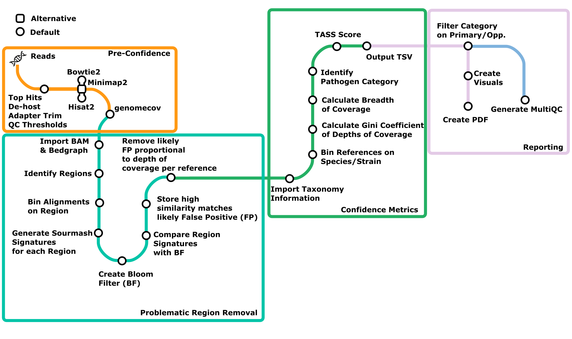
The pipeline scripts that contribute to the TASS scoring mentioned below are available here:
- Input parsing & per-reference stats - Pull alignment metrics from BAM, depth/bedgraph, and FASTA files (
match_paths.py) - Conflict resolution & signature comparison - Find and handle cases where reads map ambiguously to multiple organisms (
conflict_regions.py) - Score computation - Calculate individual features and combine them into a final TASS score (
optimize_weights.py)
Input Files
| File Type | What it's for |
|---|---|
BAM (.bam) | Aligned reads against the reference database; source of read counts, mapping quality, and coverage |
BEDGRAPH / Depth (.bedgraph, .depth) | Per-position coverage depth for each reference. Optional when --compare_references is active (coverage is derived from the BAM index instead of a bedgraph) |
FASTA (.fasta, .fa) | Reference genome sequences; used to build k-mer signatures for conflict detection. Required when --compare_references is active |
Match file (.tsv) | Maps accession IDs to taxonomy (taxid, organism name, description) |
| Kraken2 report (optional) | Independent taxonomic classification for cross-checking |
| HMP distributions (optional) | Human Microbiome Project abundance data for body-site context |
2. Stage 1: Input Parsing and Per-Reference Stats
2.1 BAM Processing (match_paths.py)
The BAM file is read using pysam. For each reference, we extract:
numreads- Number of primary, non-supplementary alignmentsmeanmapq- Average mapping quality across all aligned readshighmapq_fraction- Fraction of reads with MAPQ ≥ threshold (e.g., MAPQ ≥ 5)covered_regions- List of(start, end, depth)from the bedgraph
*Note: When --compare_references is active, coverage is estimated from BAM index statistics instead of a bedgraph file (see Section 3.8). Additionally, we will use the term contig interchangeably with reference accessions be they scaffolds, plasmids, contigs, or full chromosomes.
2.2 Coverage from Depth/Bedgraph
The bedgraph file is parsed into a table with columns (chrom, start, end, depth). For each reference:
covered_bases = sum of (end - start + 1) for every region where depth > 0

coverage = covered_bases / reference_length
Bedgraph is optional when
--compare_referencesis active. In that mode the pipeline tiles fixed-size windows across the reference FASTAs directly and compares them via k-mer sketches (Section 3.8). Coverage for scoring is then estimated from the BAM index statistics rather than from an external bedgraph file. If no bedgraph is supplied without--compare_references,determine_conflicts()raises aValueErrorimmediately so the user is not left with a empty results file.
2.3 Abundance Metrics (RPM / RPKM)
Computed in compute_scores_per(). Raw read counts aren't directly comparable between samples because some samples have more total reads than others, and some organisms have bigger genomes (which naturally attract more reads). RPM and RPKM normalize for these differences:
RPM  = numreads / (total_reads / 1,000,000)

RPKM = numreads / ((total_reads / 1,000,000) × (reference_length / 1,000))
2.4 MAPQ Normalization
From utils.py::normalize_mapq(). This rescales mapping quality to a 0 - 1 range:
The result is clipped to [0, 1] to handle any out-of-range values.
3. Stage 2: Conflict Region Detection (conflict_regions.py)
3.1 What This Stage Does
Closely related organisms (e.g., E. coli vs Shigella) share large regions of their genomes. This means reads from one organism can legitimately align to the other. This is called cross-mapping, and it inflates the apparent confidence for organisms that aren't really there.
This step finds those shared regions and removes a proportional share of ambiguous reads before scoring.
3.2 Region Merging
Raw bedgraph intervals are merged into larger contiguous regions using merge_bedgraph_regions(). The default strategy ("jump") groups adjacent intervals when:
- The depth change between consecutive intervals is ≤ a threshold (set automatically from the 97.5th percentile of depth)
- The gap between intervals is ≤ 10% of the reference length (editable via
--gap_allowance) - The merged group doesn't exceed
max_group_sizeintervals
The result is a smaller set of meaningful regions per reference, each described by (chrom, start, end, mean_depth).
3.3 Signature Generation
For each merged region, a sourmash MinHash signature is created from the reference FASTA sequence:
mh = MinHash(n=0, ksize=kmer_size, scaled=scaled)   # default ksize=31, scaled=100
mh.add_sequence(fasta.fetch(chrom, start, end))
sig = SourmashSignature(mh, name="ref:start-end")
- If FASTA files are available, the sequence is pulled directly from them.
- Regions shorter than
kmer_sizeare skipped (can't build a valid signature).
3.4 SBT Index and Search
Signatures are organized into a Sequence Bloom Tree (SBT) index, then each signature is searched against it:
for search_result in sbt.search(sig_query, threshold=min_threshold):
    jaccard = search_result.score    # Jaccard similarity between two regions
Any pair of regions from different references with Jaccard similarity ≥ min_threshold (default 0.2) is flagged as a potential conflict.
3.5 Conflict Group Construction
build_conflict_groups() builds a network (graph) of similar regions:
- Nodes are genomic regions
(ref, start, end). Each node represents one stretch of one organism's genome. - Edges connect regions from different organisms that look too similar (Jaccard similarity ≥ threshold). Jaccard similarity is a simple measure of overlap: it counts how many k-mers two regions share divided by the total unique k-mers between them. A value of 1.0 means identical; 0.0 means nothing in common.
Connected components (found with a breadth-first search, or BFS) define conflict groups: clusters of regions across multiple organisms that share enough k-mer content that reads could be assigned to the wrong member.
3.6 Best-Alignment Read Removal
For each read with multi-reference alignments, build_removed_ids_best_alignment() keeps the alignment with the highest composite score and schedules the rest for removal. The score combines four terms:
Where:
- MAPQ - raw mapping quality reported by the aligner (0 - 60)
- \(w_{AS}\) - alignment-score weight (default
0.0; AS tie-breaks only when enabled) - \(N_{\text{alt}}\) - number of competing references that share at least one high-ANI window with this contig; \(w_{pen} = 50.0\) by default
- \(\Omega_{\text{ani}}\) - ANI dominance term (see below); \(w_{ani} = 10.0\) by default
ANI Dominance Term \(\Omega_{\text{ani}}\)
Before the BAM is scanned, _count_reads_per_ref() builds a fast index of the pre-removal read count for every reference from the BAM index statistics. For each competing reference that shares a high-ANI window with the current contig, we measure how much more (or less) support our contig has:
Where:
- \(A\) - the set of competing contigs that share at least one window with this contig
- \(J_{\max}(\text{contig}, \text{alt})\) - the maximum window-level Jaccard similarity observed between the contig and that competitor (from the shared-window index). Jaccard 1.0 = nearly identical sequence; 0.1 = only slightly similar
- \(N_{\text{contig}}\), \(N_{\text{alt}}\) - pre-removal read counts for the respective references (minimum 1 to avoid log(0))
- \(\log_2(N_{\text{contig}} / N_{\text{alt}})\) - the log-ratio of read counts. This is positive when our reference has more reads than the competitor (reward) and negative when it has fewer (penalty)
Worked example, O104:H4 vs Shigella: Suppose O104:H4 has 80,000 reads and a Shigella contig has 5,000, and they share a window with \(J_{\max} = 0.95\):
ani_dominance  = 0.95 × log₂(80000 / 5000)
               = 0.95 × log₂(16)
               = 0.95 × 4.0 = 3.8

score boost (w_ani=10) → +38 points for O104:H4 alignment
score penalty          → −38 points for Shigella alignment
A single high-ANI window with a 16× read-count advantage adds ≈ 38 points, decisively overcoming any MAPQ noise between the two references. Reads that align equally well to both will therefore be assigned to O104:H4.
Parameters
The actual values passed to build_removed_ids_best_alignment() differ by mode:
| Parameter | --compare_references mode | Standard (bedgraph) mode | Effect |
|---|---|---|---|
penalize_weight | 0 | 23.0 | Penalty per competing contig in \(N_{\text{alt}}\) |
as_weight | 1.0 | 0.0 | Weight on the aligner AS tag |
ani_boost_weight | 10.0 | (not used) | Scales \(\Omega_{\text{ani}}\); raise to make dominance stronger |
min_alt_count | 2 | 1 | Minimum competing alignments before removal applies |
In --compare_references mode the ANI dominance term (\(\Omega_{\text{ani}}\)) does all the heavy lifting, so penalize_weight is set to 0. In the standard bedgraph path, as_weight is disabled (0.0) and the competing-contig penalty is 23.0.
CLI flags that control removal
The weights above are internal. These match_paths.py flags are what you actually set on the command line to change, disable, or audit removal: Two of them - --no_read_removal and --taxid_removal_stats - are also exposed as pipeline parameters, so they work with nextflow run; the rest apply only when calling match_paths.py directly.
| Flag | Default | Effect |
|---|---|---|
--dominance_protect_ratio <float> | 2.0 | Read-count ratio (dominant ÷ runner-up) within a conflict group above which the dominant reference is fully exempt from base (min_cov) removal. Dominance is decided on the raw read count in the shared region. Lower = protect more aggressively; set 0 or a very large value (e.g. 999) to disable protection and restore unconditional base removal. |
--no_read_removal (pipeline param) | false | Disable conflict read removal entirely for scoring. Conflict regions and breadth-change stats are still computed and written to disk (reference lengths and reports stay intact), but no reads are removed: coverage, Gini, numreads and the full TASS score all derive from the complete original alignment set. |
--skip_read_removal_scoring | off | Identical in effect to --no_read_removal; kept as the original spelling. --no_read_removal is the clearer name and is preferred for new commands. |
--taxid_removal_stats (pipeline param) | true | In addition to the standard removal_stats.xlsx, write a taxid-aggregated removal_stats_by_taxid.xlsx in which accessions are grouped by taxid. Requires --match (it supplies the accession → taxid mapping). On by default in the pipeline; pass --taxid_removal_stats false to skip it. |
On/off TASS comparison
--no_read_removal is the flag to reach for when post-removal coverage collapses and you want to know how much of the score change is removal and how much is the organism. Run the same sample twice - once normally, once with --no_read_removal - and diff the resulting TASS scores. Because conflict detection still runs, the removal_stats reports from the second run tell you exactly which reads would have been removed.
Removal protection interacts with roll-up
--dominance_protect_ratio acts at the strain level, before the LCA-aware species/genus logic in 11.1. If you are chasing under-called species in a group of near-identical strains, adjust the roll-up behaviour first; loosening the protection ratio changes which strain wins, not whether the species survives.
3.7 Comparison Metrics (Δ Breadth)
After read removal, compare_metrics() calculates how much each reference changed. The results are written to the conflict-comparison xlsx/csv. Each row represents one reference and includes:
Core removal metrics (always present):
| Column | Formula | Meaning |
|---|---|---|
Δ All | \(N_{\text{total}} - N_{\text{pass}}\) | Number of reads removed |
Δ All% | \(100 \times N_{\text{removed}} / N_{\text{total}}\) | Percentage of reads removed |
Δ⁻¹ Breadth | \(B_{\text{post}} / B_{\text{pre}}\) | Fraction of genome breadth that survived removal |
Abundance metrics (pre- and post-removal, so downstream scoring can see the delta):
| Column | Formula |
|---|---|
RPKM Pre | \(N_{\text{pre}} \;\big/\; \big(\tfrac{R_{\text{total}}}{10^6} \times \tfrac{L}{10^3}\big)\) |
RPKM Post | Same formula using \(N_{\text{post}}\) |
RPM Pre | \(N_{\text{pre}} \;\big/\; \big(R_{\text{total}} / 10^6\big)\) |
RPM Post | Same formula using \(N_{\text{post}}\) |
Where \(N_{\text{pre}}\) and \(N_{\text{post}}\) are read counts before and after removal, \(R_{\text{total}}\) is the total reads in the BAM, and \(L\) is the reference length in bp.
Shared-window ANI summary (populated when --compare_references is active; derived from compute_shared_window_stats()):
| Column | Meaning |
|---|---|
Shared Windows | Number of tiled windows on this reference that overlap at least one window on another reference |
Conflicting Refs | Count of distinct other references sharing at least one window |
Mean Shared ANI | Average Jaccard similarity across all shared windows (proxy for ANI; 0→1) |
Max Shared ANI | Highest single-window Jaccard seen for this reference - flags the most similar competitor |
Shared BP | Approximate total base-pairs covered by shared windows (windows may overlap) |
Δ⁻¹ Breadth and Δ All% are passed directly into the minhash score (see Section 7). The ANI summary columns are informational in the xlsx but their per-window Jaccard values feed the ANI dominance term \(\Omega_{\text{ani}}\) during read removal (Section 3.6).
3.8 Shared-Window Mode (--compare_references)
When --compare_references is passed to match_paths.py, an alternative and more thorough conflict detection approach is used. Rather than sketching merged bedgraph regions, the pipeline tiles fixed-size windows across every reference FASTA and compares them directly to find shared sequence.
How it works
- Tiling - Each reference FASTA is divided into windows of
--window_sizebp (default: 900,000 bp) with a step of--step_sizebp (default: 900,000 bp; set towindow_size/2for 50% overlap). Windows with more than 5% N-bases are skipped. - Sketching - Each window is converted to a MinHash signature (k-mer size 31, scaled 200 by default).
- Pairwise search - A
ProcessPoolExecutoris used to compare all query windows against all target windows from other FASTAs. Pairs with Jaccard ≥jaccard_threshold(default 0.10) are recorded as shared.
Performance design
report_shared_windows_across_fastas() is optimised to minimise inter-process communication overhead at scale:
- Worker initializer - Target window hash-sets are sent to each worker process once via the pool initializer (
_init_search_worker). They are deserialized and stored in a module-level dict (_SEARCH_WORKER_TARGETS), keyed by FASTA label. Subsequent job submissions carry only the query chunk, so the targets are never pickled again on a per-job basis. - Frozenset Jaccard - Similarity is computed with Python's native
frozenset &intersection (C-level), not viaMinHashobjects. This avoids Python-object construction overhead on every comparison: \(J = |A \cap B| / |A \cup B|\) where \(A\) and \(B\) arefrozensets of hash values. An early-exit is applied when \(|A \cap B| = 0\). - Intra-FASTA skip - Same-FASTA comparisons are skipped in \(O(1)\) by checking the FASTA label key before entering the inner loop.
- Job granularity - One job per query chunk (chunk size = ceil(N_queries / n_workers)), compared to the earlier approach of N_tiles × chunk jobs. This reduces scheduler overhead for large databases.
Parameters
| CLI flag | Default | Effect |
|---|---|---|
--window_size | 900,000 | Window width in bp |
--step_size | 900,000 | Step between window starts; window_size/2 gives 50% overlap |
--min_threshold | 0.4 | Jaccard threshold for the region-based (non-window) path |
--compare_references | off | Enable this mode |
Note: The bedgraph (
-b) is not required when--compare_referencesis active. The pipeline infers coverage from BAM index statistics instead. The FASTA files (-f) are required because windows are built from reference sequence.
3.9 ANI Matrix Generation
generate_ani_matrix() builds an organism-level Average Nucleotide Identity (ANI) matrix:
- Composite signatures are built per taxid from all its accessions
- Pairwise ANI is estimated from MinHash containment between organism signatures
- The result is written to
organism_ani_matrix.csvas a symmetric matrix
3.10 Pre-Removal Read Count Index (_count_reads_per_ref)
Before any reads are removed, _count_reads_per_ref() builds a dict of {reference: read_count} for every contig in the BAM. It uses the BAM index statistics (pysam.AlignmentFile.get_index_statistics()) which is an O(N_references) operation, meaning no reads have to be iterated over. If the index is unavailable, it falls back to a full single-pass scan.
This index is what enables the \(N_{\text{contig}} / N_{\text{alt}}\) ratio inside the ANI dominance term \(\Omega_{\text{ani}}\) (Section 3.6).
3.11 Shared-Window Conflict Summary (compute_shared_window_stats)
After the shared-window search, compute_shared_window_stats() aggregates the per-window results into a per-reference summary that is stored in the comparison xlsx (Section 3.7). For each reference it computes:
| Field | Computation |
|---|---|
n_shared_windows | len(windows) - count of tiled windows on this ref that have at least one match |
n_conflicting_refs | len({w.alt_contig for w in windows}) - distinct competitors |
mean_window_jaccard | statistics.mean([w.jaccard for w in windows]) |
max_window_jaccard | max(w.jaccard for w in windows) |
shared_bp | sum(w.end - w.start for w in windows) (windows may overlap; approximate) |
max_window_jaccard is the value used as \(J_{\max}\) in the ANI dominance formula, so it directly affects which organism "wins" when reads are ambiguous (Section 3.6).
3.12 Reference Exclusion, Removal Reporting and Control Samples
Three groups of match_paths.py flags sit alongside the removal machinery. They do not change the TASS formula, but they change which references reach it and what auditing output is produced.
Description-based exclusion
| Flag | Default | Effect |
|---|---|---|
--exclude_descriptions <regex> [...] | none | One or more regex patterns matched against the reference descriptions taken from --match. Any accession whose description matches any pattern is dropped from the analysis and its reads discarded. Passing the flag with no patterns filters nothing, as does omitting it. |
This runs before conflict detection, so excluded accessions never compete for reads. The usual targets are database entries that are technically valid references but scientifically noisy - unplaced scaffolds, organelle sequences, plasmid-only records:
Patterns are ordinary Python regexes, so anchor them ('^Homo sapiens') when a loose substring would over-match.
Removal and confusion reporting
| Flag | Default | Effect |
|---|---|---|
--report_metrics | off | Compute per-organism TP/FP metrics against ground-truth read IDs. Emits a JSON file plus an stdout table with per-organism TASS, TP/FP status, overall precision / recall / F1, and a threshold sweep showing what percentage of TPs and FPs pass at each TASS cutoff. Requires ground truth (--abu_file or --apply_ground_truth). |
--report_confusion_xlsx | off | Write an XLSX containing confusion-matrix statistics and the false-positive reads that survived removal. |
--confusion_xlsx <path> | <output_dir>/alignment_confusion_report.xlsx | Output path for the report above. |
These are benchmarking aids: --report_metrics is what you use when tuning weights against a known mock community, and the confusion XLSX is the drill-down for which reads are responsible for a false positive that removal did not clear.
Control samples
match_paths.py can compare a sample against previously scored control runs. Controls are supplied as the JSON output of an earlier match_paths.py run, one file per control sample.
| Flag | Default | Effect |
|---|---|---|
--negative_controls <json> [...] | none | One or more negative-control JSONs. Organisms whose TASS / read counts fall within --control_fold_threshold of the controls are flagged within_negative. |
--positive_controls <json> [...] | none | One or more positive-control JSONs. Used for the spark-bar comparison in the report. |
--control_fold_threshold <float> | 2.0 | Fold-change cutoff for the negative comparison: if sample TASS ÷ max(negative TASS) < threshold, the organism is flagged within_negative. |
--control_type <positive\|negative> | none | Mark this sample as a control. Recorded in the output JSON metadata as control_type. Omit for ordinary samples. |
--missing_pos_levels <level> [...] | toplevelkey | Hierarchy level(s) at which to detect missing positive controls. One or more of toplevelkey (genus), key, subkey (species). |
--hide_missing_pos_controls | off | Suppress detection and output of missing positive-control organisms entirely. |
--insilico_controls <json> [...] | none | One or more JSONs from in-silico simulated control samples, used to compare simulated vs real TASS scores and read counts per organism. See In-Silico Simulation. |
At pipeline level these are wired up from the samplesheet's positive / negative columns rather than set by hand; see Samplesheet. The flags above are the direct interface for running match_paths.py outside Nextflow.
4. Stage 3: Score Computation (optimize_weights.py)
All component scores are computed in compute_scores_per() and combined in compute_tass_score().
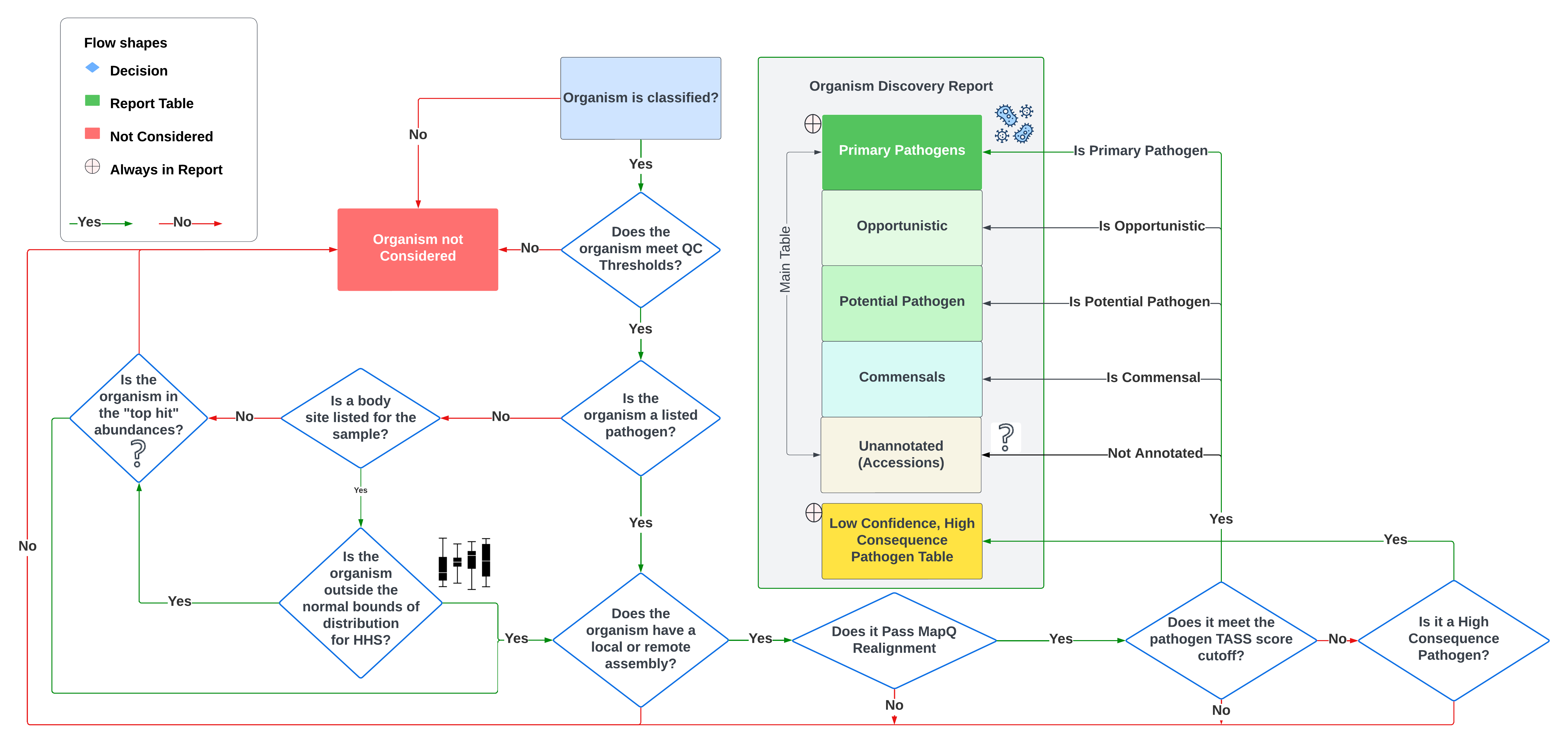
Top hits decision tree (feeds into which organisms reach the scoring stage):
5. Component 1: Breadth Log Score (Genome Coverage)
5.1 What It Measures
The breadth score captures how much of the reference genome has at least one read aligned to it. If reads are spread across the genome, that's a good sign the organism is genuinely present. If reads pile up in just one spot, it's more likely cross-mapping or contamination.
This fraction is passed through a sigmoid curve to produce a 0 - 1 confidence value.
5.2 Sigmoid Function
A sigmoid is an S-shaped curve that smoothly converts any input value into a number between 0 and 1. Think of it like a dimmer switch: instead of flipping abruptly from "off" to "on," it gradually ramps up. We use it here because we don't want the score to jump from 0 to 1 the instant coverage crosses a threshold. We want it to ramp up smoothly instead.
Defined in breadth_score_sigmoid():
Where:
- \(c\) = the coverage fraction (covered_bases / reference_length). This is just "what percentage of the genome has at least one read on it?" It ranges from 0 (nothing covered) to 1 (everything covered).
- \(m\) = the midpoint, meaning the coverage level at which the sigmoid outputs 0.5, meaning "we're 50/50 on whether this is real." Default is 0.01 (i.e., 1% of the genome covered).
- \(s\) = the steepness, which controls how quickly the curve transitions from low confidence to high confidence around the midpoint. A higher number makes the jump sharper. Default is 12,000.
- \(e\) = Euler's number (~2.718), just a mathematical constant that gives the curve its smooth S-shape.
Overflow protection: If \(s \cdot (c - m) \geq 50\), the function returns 1.0. If \(\leq -50\), it returns 0.0.
5.3 MAPQ Scaling
Low mapping quality (MAPQ ≈ 0) suggests reads are aligning ambiguously. The aligner found more than one place each read fits about equally well, so we cannot be confident it came from this organism rather than one of the others. When most reads have low MAPQ, we scale the breadth score down to reflect that uncertainty:
Where \(p\) (the exponent) = mapq_breadth_power (default: 2.0). Squaring the high-MAPQ fraction means that if, say, only 70% of reads are high-quality, the penalty is 0.7² = 0.49, which is a meaningful reduction. This makes the score more conservative when read quality is mixed.
5.4 Final Breadth Log Score
Example: Coverage = 15%, midpoint = 0.01, steepness = 12,000, 90% of reads have high MAPQ:
Where \(c\) comes from at species/genus level. At the strain level \(c\) is simply covered bases ÷ reference length. At the species and genus levels it is subject to the roll-up overrides in 11.2. In particular it can be replaced by a maximum across member accessions, which is size-gated to avoid a single small scaffold standing in for a whole genome (11.3). Because the sigmoid saturates by ~1.5 % coverage, this input is worth checking first when a species breadth score looks implausibly high next to its reported
Breadth %.
5.5 Tunable Parameters by Sample Type
| Sample Type | Midpoint | Steepness | Why |
|---|---|---|---|
| Standard | 0.01 | 12,000 | 1% coverage = moderate confidence |
| Sterile/Blood | 0.0005 | 50,000 | Even 0.05% coverage is meaningful in sterile sites |
MAPQ score sigmoid curve:

6. Component 2: Gini Coefficient (Coverage Uniformity)
Inspiration for Gini is derived from a paper that used gini to determine gene expression information from GeneGini (DOI: 10.1016/j.cels.2018.01.003).
6.1 What It Measures
The Gini score measures how evenly reads are spread across the genome. If an organism is truly present, reads should appear across many different genomic positions, not just cluster in one conserved region.
The pipeline inverts the classical Gini coefficient so that uniform coverage → high score and clumped coverage → low score.
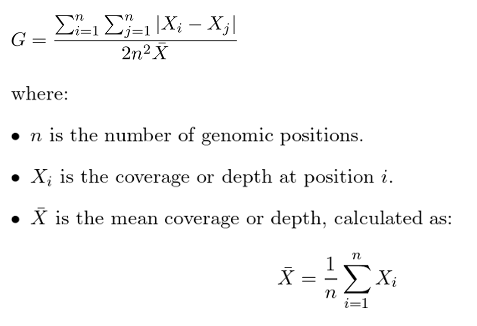
Coverage distribution examples:
| Low Confidence (clumped) | Medium | High Confidence (uniform) |
|---|---|---|
 |  |  |
6.2 Step-by-Step Computation
The full computation lives in getGiniCoeff() and has five sub-steps.
Step 1: Build a Transformed Coverage Histogram
Each region's depth is log-transformed to reduce the effect of extreme outliers. Imagine one region has a depth of 10,000 while most are around 10. Without the log transform, that one outlier would dominate the calculation. The log squashes those extremes:
Here, \(d_i\) is the raw depth at position \(i\), and \(d'_i\) is the transformed (compressed) version. The "+1" inside the log prevents taking log of zero (which is undefined). Uncovered bases get \(\log_{10}(1 + 0) = 0\).
A histogram is then built that maps each transformed depth value to the number of bases at that depth.
Step 2: Compute Raw Gini from the Lorenz Curve
The Gini coefficient is borrowed from economics (where it measures wealth inequality) and repurposed here to measure how unevenly reads are distributed across the genome. The idea: if coverage is perfectly even everywhere, Gini is 0. If all coverage is piled into one tiny spot, Gini approaches 1.
To calculate it:
- Sort coverage values from lowest to highest
- Build a Lorenz curve, which is a line that shows "what fraction of total coverage is accounted for by the bottom X% of genome positions?" In a perfectly equal world, the bottom 50% of positions would hold 50% of coverage. In practice, low-coverage positions hold very little.
- Measure the area under the Lorenz curve (\(A_L\)) using a standard trapezoid method:
Here \((x_i, y_i)\) are the Lorenz curve points, where \(x_i\) is the cumulative fraction of bases and \(y_i\) is the cumulative fraction of total coverage at that point.
\(G_{\text{raw}}\) falls in the range [0, 1]: 0 means perfectly uniform coverage, 1 means maximally unequal (all reads in one spot).
Step 3: Invert and Scale the Raw Gini
Since a low raw Gini means uniform coverage (which is a good sign), we flip and scale it so that uniform coverage gives a high score:
Where \(\alpha\) (alpha) is a scaling multiplier set to 1.8 by default. Setting it above 1.0 means that even moderately uniform distributions can reach the maximum score of 1.0. The square root softens the transformation so that small improvements in uniformity still get meaningful credit. The clamp(…, 0, 1) at the end ensures the result never goes below 0 or above 1. Examples:
- \(G_{\text{raw}} = 0\) (perfectly uniform) → \(G_{\text{transformed}} = \min(1.8, 1.0) = 1.0\)
- \(G_{\text{raw}} = 0.9\) (very clumped) → \(G_{\text{transformed}} = 1.8 \times \sqrt{0.1} \approx 0.57\)
Step 4: Length-Based Scaling Factor
Larger genomes need more reads to achieve uniform coverage, so it's harder to get a good Gini score for a big genome. To compensate, we give a bonus that scales with genome size. We use a log scale so the bonus grows gradually rather than exploding for very large genomes:
Where:
- \(L\) = the genome length (in base pairs)
- \(L_{\text{base}}\) = a baseline genome length (default: 500,000 bp). Genomes shorter than this get no bonus.
- \(L_{\max}\) = a length cap (default: 10⁹ bp) to prevent absurdly large genomes from getting too much of a boost.
- \(R\) = the reward factor (default: 2), which controls how generous the bonus is. Higher R = more reward for larger genomes.
Step 5: Positional Dispersion Factor
This measures how spread out the covered regions are physically along the genome. Even if the depth of coverage is uniform, we want reads scattered across many different locations and not all clumped in one contiguous block. Think of it like this: if you're checking whether someone actually read a whole book, you'd be more convinced if they could talk about many passages from every chapter with general detail instead of having a highly detailed summary of just one chapter.
Breaking this down:
- First, we find the midpoint of each covered region: \((s_i + e_i) / 2\), where \(s_i\) is the start position and \(e_i\) is the end position of region \(i\).
- \(\bar{m}\) (m-bar) is the average midpoint across all \(n\) regions. It tells us where the "center of mass" of coverage is.
- \(\sigma^2\) (sigma squared) is the variance of those midpoints, meaning how spread out they are from the average. If all regions are near the same spot, variance is low. If they're scattered across the genome, variance is high.
- \(L^2/12\) is the key normalization term. It represents the maximum possible variance you'd see if regions were spread out as evenly as possible (uniformly distributed) across a genome of length \(L\). This comes from a well-known statistical fact: a uniform distribution over any range [0, L] has a variance of exactly L²/12. By dividing the actual variance by this, we get a ratio that tells us "how spread out are our regions compared to the best-case scenario?" The denominator has been shown with some slight benchmarking to be sufficient for most genomes but could use some additional tuning in the future.
- \(D\) (the Dispersion factor) is the square root of that ratio, which brings it back to the same scale as the original positions. \(D\) falls in the range [0, 1]: a value near 0 means everything is clustered together, while a value near 1 means the regions are spread out almost as well as theoretically possible.
Step 6: Final Gini Score
Where \(\beta\) (beta) is the dispersion weight (default: 0.5). It controls how much the positional spread of reads (the \(D\) factor from Step 5) influences the final Gini score. At 0.5, if regions are perfectly spread out (\(D = 1.0\)), the score gets a 50% boost (multiplied by 1.5). If \(\beta\) were 0, dispersion would be ignored entirely. If \(\beta\) were 1.0, perfect dispersion would double the score. The default of 0.5 strikes a balance: spatial spread matters, but it's not the dominant factor.
Example: Moderate uniformity (\(G_{\text{raw}} = 0.3\)), genome length 5 Mbp, well-spread regions (\(D = 0.7\)):
G_transformed  = 1.8 × √(0.7) ≈ 1.0 (clamped to 1.0)
S_length       = 1 + 2 × log10(5,000,000 / 500,000) = 1 + 2 × 1 = 3.0
Dispersion     = 1 + 0.5 × 0.7 = 1.35
Final          = min(1.0, 1.0 × 3.0 × 1.35) = 1.0 (clamped to 1.0)
7. Component 3: Minhash Reduction (Signature-Based Uniqueness)
7.1 What It Measures
The minhash component asks: how much did this organism's signal change after we removed cross-mapped reads?
An organism that loses most of its reads during conflict resolution probably wasn't genuinely present, because those reads belonged to something else. An organism that retains its reads is more likely real.
7.2 Raw Minhash Score
The conflict detection pipeline produces per-reference metrics at the species level. Two values are key:
Δ⁻¹ Breadth(\(B_r\)): The ratio of post-removal breadth to pre-removal breadth. Think of it as "what fraction of genome coverage survived after we removed ambiguous reads?" A value of 1.0 means no breadth was lost, which is good because it means the signal was all unique. A value of 0.5 means half the coverage came from reads that could've belonged to a different organism (concerning).Δ All%(\(\Delta\%\)): The percentage of total reads that were removed during conflict resolution. The Δ (delta) here means "change," specifically how many reads changed by being removed.
The raw minhash score blends two retention signals, breadth retention and read retention, to differentiate true positives from false positives, particularly within high-ANI conflict groups (e.g. E. coli vs Shigella) where \(B_r\) alone is nearly identical for every member:
Δ⁻¹ Breadth(\(B_r\)): fraction of genome breadth surviving conflict removal (0 - 1).- Read retention (\(R_r\)): fraction of reads surviving conflict removal, i.e.
Pass Filtered Reads / Total Reads.
Read retention is weighted more heavily (70%) because it differentiates conflict-group members much more cleanly: the dominant true-positive organism retains most of its reads during removal, while false-positive relatives lose the majority of theirs.
Example, O104:H4 vs Shigella in the same conflict group:
O104:H4  (TP):  Br=0.12, read_retention=0.85  →  0.30×0.12 + 0.70×0.85 = 0.631
Shigella (FP):  Br=0.12, read_retention=0.30  →  0.30×0.12 + 0.70×0.30 = 0.246
Both organisms have the same \(B_r\) (they share similar genome breadth reduction in the high-ANI group), but their read-retention scores clearly separate them.
Fallback (no comparison data available):
When conflict comparison data isn't available, we fall back to a simpler estimate based on how many reads the organism has relative to the total:
Where rpm_confidence is a sigmoid over the fraction of total reads (\(f_{\text{reads}}\)). The very steep sigmoid (steepness = 50,000) acts almost like a switch: if the organism has more than a tiny fraction of reads (above 0.01%), confidence jumps to ~1.0; below that, it drops to ~0:
7.3 Confidence Gating
Before the minhash score is used, it's "gated" by a coverage confidence factor. Think of a gate as a checkpoint: if an organism doesn't have enough genome coverage, we don't trust its minhash score regardless of how good it looks. This prevents organisms with very sparse coverage from getting artificially inflated scores:
Here \(w_b\) and \(w_g\) are weights that control how much the breadth sigmoid vs. the Gini score contribute to the gate. By default \(w_b = 1.0\) and \(w_g = 0.0\), so gating is based purely on breadth (genome coverage).
Note: The value stored as
minhash_reductionis the confidence value, not the raw minhash score itself. This means the minhash component represents how confident we are that the organism's alignment signal is real, and that confidence is driven mainly by whether the organism has meaningful genome breadth.
At the group (species/genus) levels the gate is the product of three factors, all of which must be healthy for minhash to survive:
Note that breadth_sigmoid(c) here uses the same \(c\) as the breadth component, so an inflated group coverage does not just raise breadth. It simultaneously unlocks the minhash term, and the two are the two largest weights in the default profile. This coupling is why a single bad coverage value moves TASS so far; see 11.3 for the guard and the worked P. vivax example.
7.4 Low-Read Penalty with Coverage Bypass
Organisms with very few reads relative to the total are more likely to be false positives, so their minhash_confidence is scaled down by a coverage-aware penalty. Rather than applying the penalty at full strength regardless of coverage evidence, it is faded out when the organism has solid genome breadth. This keeps a well-covered dominant organism from being dragged down by the global read-fraction sigmoid:
where mapq_norm \(= \min(1.0, \text{meanmapq} / 60)\). The additional MapQ bypass term (0.20 × mapq_norm) fades the penalty further when reads are high-quality. A high-MAPQ organism with few reads, such as a rare pathogen in a sterile-site sample, should not be penalised as harshly as a low-MAPQ scatter hit.
Where rpm_weight is a steep sigmoid over the fraction of total reads:
and cov_conf = breadth_sigmoid(coverage).
Effect at different coverage levels (with mapq_norm = 0, i.e. low MAPQ):
cov_conf | \(w_{\text{pen}}\) | Penalty at rpm_weight=0.1 | Meaning |
|---|---|---|---|
| 0.95 (100% breadth) | 0.017 | ×0.998 (≈ none) | Dominant organism, penalty bypassed |
| 0.50 (moderate) | 0.175 | ×0.843 (−16%) | Moderate dampening |
| 0.10 (sparse) | 0.315 | ×0.717 (−28%) | Full penalty applies |
When mapq_norm = 1.0 (MAPQ 60), the effective coverage bypass is raised by 0.20, reducing \(w_{\text{pen}}\) further at every coverage level.
This ensures that a high-confidence organism like O104:H4, which spans the full genome, is never unfairly penalised simply because its read fraction is computed against total sample reads that include many other organisms.
7.5 RPM-Normalised Minhash Reduction (Multi-Member Groups)
Within each parent group (organisms sharing the same toplevelkey, i.e. the same species or taxid group), minhash scores are further adjusted based on each organism's share of total RPM within that group. This is the final normalisation step and runs after the confidence gate and read-penalty.
Solo organisms (only member in their group)
A single organism in its group gets an exclusivity boost: the gap between its current minhash_reduction and the coverage-gate ceiling is partially filled, proportional to rpm_confidence_weight:
The minhash_confidence ceiling ensures a low-coverage solo organism can't inflate itself beyond what its coverage evidence supports.
Multi-member groups: dominant organism
The member with the highest RPM in the group is boosted toward its coverage-gate ceiling rather than scaled down. This is the key change for high-ANI groups like O104:H4 vs Shigella:
Where rpm_share \(= \text{rpm}_{\text{this}} / \sum_{\text{group}} \text{rpm}\).
Example: O104:H4 has 60% of group RPM, raw_minhash = 0.90, minhash_confidence = 0.95:
gap     = 0.95 − 0.90 = 0.05
boost   = 0.05 × 0.60 = 0.03
adjusted = min(0.95, 0.90 + 0.03) = 0.93   ← was 0.72 before this change
Multi-member groups: losing organisms
All non-dominant members are penalised using a two-part multiplicative scale:
Part 1, the RPM-share floor:
The floor of 0.10 (reduced from the previous 0.30) prevents partial false positives from retaining an inflated minhash score. With a 10% floor, Shigella at 8% RPM share gets a base scale of ≈ 0.17.
Part 2, the coverage-ratio penalty:
If the dominant organism has 20% genome coverage and this organism only has 4%, the coverage ratio is 0.20, giving cov_scale = 0.25 + 0.75×0.20 = 0.40. This extra penalty captures the case where a low-coverage organism has a similar RPM share simply because its reads all piled into one conserved region.
Full worked example, Shigella vs O104:H4:
rpm_share  = 0.21   cov = 8%   top_cov = 20%

base_scale = 0.10 + 0.90 × 0.21 = 0.289
r_cov      = 8 / 20 = 0.40
cov_scale  = 0.25 + 0.75 × 0.40 = 0.55
scale      = 0.289 × 0.55 = 0.159

adjusted   = 0.90 × 0.159 = 0.143   ← was 0.72× before
The combined effect is that in a high-ANI conflict group, the organism with the most reads and broadest coverage is strongly promoted, while relatives (Shigella, other E. coli strains) have their minhash contribution cut to a small fraction of its naive value.
8. Additional Scoring Components
8.1 HMP Percentile (Body-Site Abundance Context)
This compares the observed abundance to what the Human Microbiome Project found for this organism at the relevant body site. If an organism is at typical abundance for that site, it gets a neutral score. Unusually high or low abundance is flagged.
Breaking this down:
- \(f_{\text{obs}}\) is the observed fraction of reads belonging to this organism, which is simply its read count divided by the total read count.
- \(\mu_{\text{HMP}}\) (mu) is the average abundance for this organism at this body site, according to the Human Microbiome Project data.
- \(\sigma_{\text{HMP}}\) (sigma) is the standard deviation of that abundance, which tells you how much variation is normal.
- \(z\) is the z-score: how many standard deviations away from normal our observation is. A z-score of 0 means "exactly average," +2 means "well above average," and -2 means "well below average."
- \(\Phi(z)\) (Phi of z) converts the z-score into a percentile on a bell curve. For example, a z-score of 0 gives the 50th percentile; a z-score of +2 gives the 97.5th percentile.
The base percentile is then adjusted based on how far from normal it is:
| Z-score range | Adjusted percentile | What it means |
|---|---|---|
| \(z < -1.0\) | \(P_{\text{base}}^2\) | Penalize - below typical |
| \(-1.0 \leq z \leq 1.0\) | \(P_{\text{base}}\) | Neutral - near expected |
| \(1.0 < z \leq 2.0\) | \(1 - (1 - P_{\text{base}})^{1.5}\) | Boost - above typical |
| \(z > 2.0\) | \(1 - (1 - P_{\text{base}})^{2}\) | Strong boost - well above typical |
8.2 Plasmid Score
Within each species, strains are compared by their plasmid coverage. Calc. in match_paths.py.
Absolute quality (does this plasmid have good coverage?):
Where \(B_{\text{plasmid}}\) is the breadth sigmoid score for the plasmid's coverage and \(G_{\text{plasmid}}\) is the Gini coefficient for the plasmid's depth distribution. The square root of this product is called a geometric mean. It is a way of averaging two values that requires both of them to be decent. The reason we use the geometric mean is because it accounts for means in extreme value scenarios i.e. there is a more likely scenario that a small plasmid will either have no coverage or super good coverage. If either breadth or uniformity is near zero, the geometric mean is poor. You can't fake a good plasmid score with good breadth of coverage but terrible uniformity, or vice versa.
Relative disparity (how does this strain compare to others in the same species?):
In other terms: when there are multiple strains of the same species (matched from their shared species level taxid), we compare each strain's plasmid coverage (\(c_{\text{strain}}\)) and read count (\(r_{\text{strain}}\)) against the best strain in the group (\(c_{\max}\) and \(r_{\max}\)). Coverage gets 70% of the weight and read count gets 30%. If this is the only strain with a plasmid, there's nothing to compare against, so it gets a 1.0.
Final plasmid score:
Strains with no plasmid accessions receive plasmid_score = 0. This is not a penalty so that we don't strains/species that lack plasmids in the database/references.
8.3 Low-Abundance Confidence
This is a sigmoid curve applied in log₁₀-RPM space that gives credit to organisms that have a meaningful number of reads per million, even when the absolute read count is small. It's especially useful for sterile-site or blood samples where you don't expect many reads from any organism, but even a few reads can be clinically significant.
Where \(s\) = steepness (default: 2.0) and \(m\) = RPM midpoint (default: 5.0).
8.4 K2 Disparity Score
Compares the pipeline's species-level classification against Kraken2's (or Centrifuge if enabled instead) classification. If Kraken2/Centrifuge assigns reads to a different genus, this reduces confidence. Disabled by default (k2_disparity_score_weight = 0).
8.5 DIAMOND Identity
Average amino acid identity from a DIAMOND BLASTX protein alignment, weighted by CDS count. Provides protein-level confirmation of the taxonomic assignment. Disabled by default (diamond_identity = 0). We have not tested this since v1.0 so consider it less reliable of a tool to implement. The associated modules are still functional, however.
9. Final TASS Score Formula
9.1 The Core Weighted Sum
Computed in compute_tass_score(). The final score is simply a weighted sum: each component score (\(x_i\)) is multiplied by its relative weight (\(w_i\)), and then they're all added together and clamped between 0 and 1. Components with higher weights have more influence on the final result:
Expanded:
9.2 Default Weights
| Component | Weight | CLI Flag | Type |
|---|---|---|---|
breadth_log_score | 0.27 | --breadth_weight | included |
minhash_reduction | 0.31 | --minhash_weight | included |
gini_coefficient | 0.42 | --gini_weight | included |
hmp_percentile | 0.00 | --hmp_weight | included |
disparity | 0.00 | --disparity_weight | included |
mapq_score | 0.00 | --mapq_score | included |
k2_disparity_score | 0.00 | --k2_disparity_score_weight | included |
diamond_identity | 0.00 | --diamond_identity | included |
plasmid_bonus_weight | 0.00 | --plasmid_bonus_weight | bonus |
What if all weights don't add up to 1.0? The three active primary weights (breadth=0.27, minhash=0.31, gini=0.42) sum to 1.0, which is the intended normalization. The plasmid bonus and abundance confidence weights sit outside this normalized pool and are additive on top of the base sum. This is intentional. The final score is clamped to \([0, 1]\) at the end, so overshooting is fine. It allows components to reinforce each other when the support for an organism is strong.
9.3 Additive Modifiers
Plasmid bonus (applied after the base sum):
Where \(w_{\text{plasmid}}\) = plasmid_bonus_weight (default: 0.0, which disables it).
This can also work with additional additive modifiers to be added in the future.
9.4 Multiplicative Abundance Gate (Optional)
When --abundance_gate (not recommended for most samples) is enabled, the full score is multiplied by the abundance confidence sigmoid. This collapses scores for organisms with very low read fractions:
Note: This is exclusive with the additive plasmid_bonus_weight approach.
9.5 Power Transform (Optional)
When score_power isn't set to the default of 1.0, a power transform reshapes the score distribution. This is useful for adjusting how "generous" or "strict" the final scores are. A power less than 1 rises low scores (making the system more lax), while a power greater than 1 would push low scores even lower (more conservative):
Where \(p\) = score_power. Some examples:
- \(p = 0.5\): score 0.09 → 0.30, score 0.95 → 0.97 (rises low scores, making borderline organisms more visible)
- \(p = 0.3\): score 0.09 → 0.52, score 0.95 → 0.98 (dramatically rises low scores)
- \(p = 1.0\): no change (this is the default, and the score passes through as-is)
The transform is not applied uniformly across organisms: a per-record score_power_scale derived from ANI grouping determines how much of it each organism receives. See 11.6.
9.6 Final Clamping
Full score formula diagram:

Disparity score example:

10. Full Pipeline Sequence Diagram
BAM file ──────────────────┐
                           ▼
                    ┌──────────────┐
BEDGRAPH/depth ───▶│ match_paths  │──▶ per-reference stats:
                   │   .py        │    numreads, meanmapq, coverage,
Match file ───────▶│              │    covered_regions, highmapq_fraction
                   └──────┬───────┘
                          │
          ┌───────────────┼───────────────┐
          ▼               ▼               ▼
   ┌─────────────┐ ┌────────────┐  ┌────────────────┐
   │ conflict_   │ │ optimize_  │  │ map_taxid.py   │
   │ regions.py  │ │ weights.py │  │ body_site_     │
   │             │ │            │  │ normalization   │
   │ • merge     │ │ • gini     │  │ • taxonomy     │
   │   bedgraph  │ │ • breadth  │  │   lookup       │
   │ • sketch    │ │ • minhash  │  │ • pathogen     │
   │   signatures│ │ • HMP      │  │   classification│
   │ • SBT search│ │ • plasmid  │  └────────────────┘
   │ • conflict  │ │ • TASS     │
   │   groups    │ │   scoring  │
   │ • read      │ └─────┬──────┘
   │   removal   │       │
   └──────┬──────┘       │
          │              │
          ▼              ▼
   comparison_df    TASS scores
   (Δ Breadth,     per organism
    Δ All%)              │
          │              ▼
          └────────▶ Final TSV Report
Extra
Example command line for running TASS calculations:
To run match_paths.py you will need 4 files minimum along with a directory of taxonomy (taxdump). Make sure you're in the bin folder and adjust paths as needed. The required files are:
- BAM file with reads aligned to the reference database
- FASTA file with reference sequences (optional but improves conflict detection)
- Bedgraph file with coverage depth per position for each reference
-
Match file mapping accessions to taxids and organism names
-
Alignment files can be generated with standard tools like Minimap2 or Bowtie2, using the same reference database that TASS will use for scoring. Example command can be:
minimap2 \
     -ax sr \
    --split-prefix Miseq_Run_A.Miseq_Run_A.dwnld.references.prefix \
    Miseq_Run_A.dwnld.references.fasta \
    Miseq_Run_A_1.fastq.gz Miseq_Run_A_2.fastq.gz \
    -L \
    -a | samtools sort | samtools view -b -h -o Miseq_Run_A.Miseq_Run_A.dwnld.references.bam
- Ensure (for speed reasons) that the reference FASTA file is indexed with
samtools faidxand that the BAM file is indexed withsamtools indexbefore running the TASS pipeline. You can runsamtools faidxandsamtools indexwith:
samtools faidx Miseq_Run_A.dwnld.references.fasta
samtools index Miseq_Run_A.Miseq_Run_A.dwnld.references.bam
- The bedgraph can be generated with
bedtools genomecovor similar. Example command:
Note: The bedgraph is not required when using
--compare_references. In that mode the pipeline tiles windows across the FASTA files directly and derives coverage from the BAM index. You can omit-bentirely from the command below if you are using--compare_references.
- The match file should be a TSV with columns:
accession,taxid,organism_name,description. This can be generated from the reference FASTA headers and a taxonomy lookup. Example:
| Acc | Mapped_Value |
|---|---|
| NC_000913.3 | 511145 |
| NC_000964.3 | 224308 |
| NC_001781.1 | 11250 |
| NC_001803.1 | 208893 |
You can also provide custom names with the --namecol option if you don't want the taxdump names to be used by default. You'll need to have the column index (0-index) added to the match file and specify the column name like --namecol 2. Example:
| Acc | Mapped_Value | Custom_Name |
|---|---|---|
| NC_000913.3 | 511145 | Escherichia coli str. K-12 substr. MG1655 |
| NC_000964.3 | 224308 | Bacillus subtilis subsp. subtilis str. 168 |
| NC_001781.1 | 11250 | Human respiratory syncytial virus |
| NC_001803.1 | 208893 | Pseudomonas aeruginosa PAO1 |
|
Finally, the TASS scoring can be run with:
match_paths.py \
       -i Miseq_Run_A.Miseq_Run_A.dwnld.references.bam \
       -o Miseq_Run_A.paths.json \
       -b Miseq_Run_A.bedgraph \
       -s Miseq_Run_A \
       -t nasal \
       --output_dir search_results \
       -f Miseq_Run_A.dwnld.references.fasta \
       -p pathogen_sheet.csv \
       -m Miseq_Run_A.merged.taxid.tsv \
       --k2 Miseq_Run_A.filtered.report \
       --taxid_removal_stats \
       --rank genus \
       --minmapq 5 \
       --compare_references \
       --taxdump taxdump \
       --platform ILLUMINA \
       --thresholds_json sampletype_best_thresholds.json
 The above command is an example and may require adjustments based on your specific file paths, sample types, and desired parameters. Not all of these args are required as well, so you can omit those that don't apply to your use case. For instance, if you don't have Kraken2/Centrifuge results for comparison, you can leave out the
 --k2 argument.
The output will be in JSON format, which can be generated downstream as ODR and TSV with:
create_report.py \
  -i Miseq_Run_A.paths.json \
  -u Miseq_Run_A.organisms.report.txt \
  -o Miseq_Run_A.organisms.report.pdf \
  --show_potentials \
  --rank genus
11. Aggregation Levels
TASS answers two related but distinct questions: how strong is the evidence for this exact reference or strain, and if the strain cannot be resolved, how strong is the evidence for the containing species or genus? Closely related references share large portions of their genomes, so one read may align equally well to several strains. That ambiguity should reduce confidence in an exact strain, but it should not automatically erase valid evidence for the shared species or genus. Sections 11.4 - 11.8 cover the conceptual model; 11.1 - 11.3 cover the mechanics.
Scores are computed at multiple taxonomic levels:
- Accession level - Raw per-reference statistics
- Strain level (key) - Accessions grouped by strain; plasmid accessions are tagged and scored separately
- Species level (subkey) - Aggregated across strains; minhash comparison operates at this level
- Genus level (toplevelkey) - Highest aggregation, used for HMP lookups and final reporting. You can adjust this for higher level lookups such as order or family.
At each level, metrics are either summed (numreads, covered_bases), averaged (MAPQ), or re-computed from scratch (gini, breadth from merged regions). The toplevelkey can also be adjusted with the --rank parameter in TaxTriage.
11.1 LCA-aware read removal (species/genus)
match_paths.py resolves alignment conflicts (Section 3.6) at the strain level: a read that maps about equally well to two references is assigned to one and removed from the other. For organisms with several near-identical strains in the database, this is too aggressive once you move above the strain rank. The canonical case is three closely related Salmonella strains in a dilution series. A read that could have come from any of the three is genuinely ambiguous about which strain, but it is not ambiguous at all about the species, since all three candidates are the same species. Strain-level removal does not know that, so the strains end up eating into each other's numbers: every ambiguous read is subtracted from all but one of them. Each strain's coverage and read count drops, and all three can land below the reporting cutoff even though the species is obviously present.
To fix this, match_paths.py now builds accession → species (subkey) and accession → genus (toplevelkey) rollup maps from the taxdump before conflict removal runs, and passes them into determine_conflicts. Reads that are ambiguous only among members of the same species (or genus) are kept at that level. This is called LCA-aware removal, after the lowest common ancestor: the deepest point in the taxonomy that every one of a read's candidate references sits underneath. If that point is at or below the rank being scored, the read is not ambiguous about that rank, so it stays. For each accession the conflict step emits, alongside the strain-level numbers, covered bases and surviving read counts under species-LCA and genus-LCA removal (Covered BP Subkey/Toplevelkey, Pass Filtered Reads Subkey/Toplevelkey). These per-taxid removal numbers are written to alignment/<sample>_removal_stats_by_taxid.xlsx.
11.2 Species/genus roll-up score overrides
When the strain rows are aggregated to species and genus, the strain-removal coverage would still understate the group. The aggregation therefore applies three overrides built from the LCA-aware columns:
- Union breadth. Species/genus breadth is measured as the union of member coverage (Σ covered-bp ÷ Σ reference length under same-rank-LCA removal), so it reflects how well the species can be told apart from other species, not how its own strains compete with each other. This overrides the strain-derived
Breadth New/Δ⁻¹ Breadthfeeding the minhash score. - Representative (best-strain) coverage. Because near-identical conspecific strains are essentially the same genome, the group's coverage is taken as the maximum per-member breadth fraction (and the max against each strain's actual post-removal coverage), not the length-weighted pool. This prevents one divergent or poorly covered member reference from diluting an otherwise ~100 % species call. It also guards against conserved cross-species regions (rRNA, housekeeping genes) being stripped by species-LCA removal and making the representative fraction look artificially low. This maximum is restricted to accessions large enough to represent the genome; see 11.3 below.
- Pre-MAPQ read count. Strain-level
numreadsonly counts reads with MAPQ ≥--minmapq(default 7). For near-identical strains most reads have MAPQ 0, meaning they are ambiguous about which strain but not about the species. Species and genus RPM/abundance therefore use the pre-MAPQ count instead (reads surviving species-LCA removal regardless of MAPQ), summed per group without double counting.
The combined effect is "MAPQ relief": e.g. in the Salmonella test, species-level effective minhash factor rises from 0.134 to 0.682, so a real species/genus call survives even when no single strain does. In the interactive report these are surfaced as the orange (species) / purple (genus) roll-up rescue markers.
A related fix injects each reference's mean conflict MAPQ into the shared-windows cluster-dominance record so the dominant-organism gate floor in optimize_weights.py activates on that path too (previously a missing value silently forced the floor to 0).
Disabling removal for comparison.
--no_read_removal(a clearer alias of--skip_read_removal_scoring) computes conflict regions and writes the stats to disk but applies no read removal to the scoring inputs, so coverage, Gini, numreads and TASS all derive from the complete original alignment set. Useful for an on/off TASS comparison when post-removal coverage is very low. See 3.6 → CLI flags that control removal for this and the related removal flags.
11.3 Size eligibility for the representative-coverage maximum
The representative-coverage override in 11.2 takes a maximum across members. The subtlety is what counts as a member: comparison_df is indexed per accession, and an accession is one BAM reference, which means one contig and not necessarily one genome. For a chromosome-level assembly those are the same thing (the single accession is the whole genome), and the maximum behaves exactly as intended. For a scaffold-level draft assembly they do not.
The failure mode this creates:
Plasmodium vivax is distributed as ~2,700 unplaced scaffolds of ~1 kb each, totalling 27 Mb. A handful of stray ONT reads land on 5 scaffolds. One ~850 bp read covers 848 bp of a 906 bp scaffold → that accession's breadth fraction is 0.936. The maximum promotes 0.936 to the coverage of the entire species, even though true species breadth is 5,060 ÷ 27,013,691 = 0.019 %.
That single value is not confined to the breadth term. agg['coverage'] is consumed four separate times in calculate_normalized_groups, so one inflated number cascades:
| Consumer | With true breadth (0.019 %) | With the scaffold maximum (93.6 %) |
|---|---|---|
breadth_log_score (5.4) | 0.000 | 1.000 |
minhash _breadth_gate (7.3) | 0.000 - gate shut | 1.000 - gate open, minhash 0 → 0.958 |
_depth_conc_penalty (6) | crushed | efficiency looks ideal |
| dominant-organism gate floor (7.4) | - | raised |
Species TASS lands at ~89 for an organism that is not present. The strain-level rows are unaffected and score correctly (2.6 - 5.0), which is the diagnostic signature: a species scoring 80+ while every one of its strains scores below 10 is this bug.
The guard. An accession may set its group's maximum only if it is large enough to plausibly stand in for the whole genome. It has to clear either of these two bars:
where \(f\) = --rep_breadth_min_frac (default 0.01, i.e. 1 % of the group's total reference length) and \(L_{\min}\) = --rep_breadth_min_len (default 50,000 bp). If no accession in a group qualifies, the group receives no representative override at all and falls back to the pooled Σ covered ÷ Σ length. Setting both to 0 restores the pre-guard behaviour.
The bars are deliberately loose. A 4.6 Mb E. coli chromosome clears both by orders of magnitude and still sets the maximum; its 5 kb plasmid at 100 % coverage does not. The three-strain Salmonella case from 11.2 is byte-for-byte unchanged (coverage 0.99, TASS 92.85 before and after).
Interaction with the contig-utilisation penalty. The Gini contig-utilisation penalty (6, step "Fix 1") exists precisely to catch "reads on 5 of 2,700 contigs", and it also multiplies into the minhash coverage gate. It was silently inert at the species and genus levels: it counted len(entries), and at those levels entries are strain records, and there is usually only one of them, so the group saw 1/1 contigs and applied no penalty. It now sums the n_contigs_total / n_contigs_covered stamped onto each member by the strain-level aggregation, falling back to len(entries) only when members carry no such annotation (i.e. at the strain level itself, where entries genuinely are contigs). P. vivax now presents as 5/2700 → penalty ≈ 0.09.
The two guards are independent and complementary: size eligibility stops the fabricated coverage value at the source, and the contig-utilisation penalty catches groups where a large accession is genuinely eligible but the reads are still concentrated on a tiny slice of it.
Verification. bin/test_rep_breadth_scaffold_fp.py reproduces the case above from the observed contig lengths and asserts both guards, the score collapse, and the E. coli / Salmonella non-regressions:
| before | after | |
|---|---|---|
| representative override | 0.9360 | none - no eligible accession |
coverage | 0.9360 | 0.000187 |
breadth_log_score | 1.0000 | 0.0000 |
minhash_reduction | 0.9580 | 0.0000 |
| contig fraction | 1/1 | 5/2700 |
| species TASS | 87.86 | 6.11 |
11.4 Why ambiguity is rank-dependent
Several references with similar read counts can mean very different things: multiple strains are genuinely present; one strain is present but its reads cross-map to relatives; the reads come from sequence conserved across the species or genus; a small conserved locus is generating a false-positive genome hit; or the database simply contains redundant near-identical references. Raw aligned-read count cannot distinguish these, which is why TASS scores coherence of evidence rather than its volume.
The key observation is that a read can be ambiguous at one rank and unambiguous at the next one up:
At the strain level, R cannot identify the correct strain. At the species level every mapping agrees on Species X, so R is perfectly good species evidence. This is why determine_conflicts builds three removal sets rather than one (11.1): a read is removed only when its ambiguity crosses the boundary of the rank being scored.
The intended outcome is a statement like "the exact strain is unresolved, but the species is strongly supported", or, when the ambiguity spans several species of one genus, "the species is unresolved, but the genus is strongly supported."
Dominance-aware removal at the strain level. Within a single rank, the two sides of a conflict are not treated as equals (Section 3.6). When two references compete for the same ambiguous reads, the pipeline does not split those reads down the middle. It works out which reference is the more likely true source and takes the reads away from the other one. The reference with the most support in a shared region is treated as that likely source. Weaker references lose a larger share of their ambiguous reads, and a reference that clearly dominates is protected from being whittled away by many small removals in a row. Without this asymmetry, a single organism that really is present would generate a cloud of relatives that all look equally confident, and every one of those relatives would be a false positive.
Conceptual poxvirus example. One poxvirus is present, but conserved reads align to several related poxvirus references:
| Reference | Raw reads | Expected interpretation after conflict handling |
|---|---|---|
| Strain A | 1,100 | broad, coherent coverage; most support retained |
| Strain B | 420 | much of the support lies in sequence shared with A |
| Strain C | 390 | much of the support lies in sequence shared with A |
| Strain D | 360 | narrow coverage in conserved loci |
| Strain E | 330 | narrow coverage in conserved loci |
| Strain F | 310 | narrow coverage in conserved loci |
Strain A should retain the strongest breadth, evenness and read support; B - F should lose confidence to the extent their support sits in shared regions. If no reference has convincing strain-specific evidence, every strain score may stay modest even while the parent taxon is well supported. None of this is poxvirus-specific. It falls out of the general shared-sequence, dominance, breadth and rank-aware logic described above.
Parent scores are recalculated, not inherited. After strain-level processing, match_paths.py groups strains into species (subkey) and genus (toplevelkey) records; calculate_normalized_groups() reconstructs aggregate evidence and the group then passes through calculate_aggregate_scores() and compute_tass_score(). A parent score is therefore not mean(child TASS) and not max(child TASS). It is TASS(reconstructed parent-level evidence), computed from parent-level retained reads, breadth, Gini, minhash retention, MAPQ reliability, abundance and sibling disparity. This is the reason weak strain resolution does not imply weak species or genus detection.
11.5 Conditional MAPQ relief at the parent rank
Low MAPQ normally reduces confidence, and rightly so, because it means the aligner could not decide where the read belonged. But at the species or genus level, low MAPQ is often caused by redundant members of the same valid group: the uncertainty is about which reference copy the read came from, not about which organism. Crushing parent breadth by that MAPQ wrongly tanks a species that is confidently present.
calculate_normalized_groups() therefore lifts the effective high-MAPQ fraction toward 1.0, but only when all three conditions hold:
- the record is a real group aggregation with union coverage engaged (a
group_covered_bp_overrideexists for this group); - the group has more than one member, so multimapping is expected;
- minhash independently confirms the genome is present (aggregated
minhash_score> 0).
where \(h\) is the raw highmapq_fraction and \(h_{\text{eff}}\) is stored as highmapq_fraction_effective and used in place of \(h\) in the breadth MAPQ scaling of Section 5.3. Redundancy is 0.5 at two members, 0.67 at three and 0.75 at four, so the relief grows slowly as the group gets larger and never exceeds what minhash independently supports.
This is not a blanket rescue. A single-member group gets no relief at all, and a group with weak minhash support gets almost none. It is the mechanism behind the Salmonella result quoted in 11.2 (highmapq_fraction 0.13, coverage 1.0, minhash 1.0 → species TASS unstuck from ~77).
11.6 ANI-aware score-power scaling
The optional power transform of Section 9.5 does not apply uniformly. match_paths.py pre-computes a per-organism score_power_scale that controls how much of the transform each record receives.
Grouping is ANI-first. When an ANI matrix is available, any two organisms whose ANI is at or above --ani_threshold are placed in the same group, and membership is transitive: if A is close to B and B is close to C, then A, B and C all end up in one group even if A and C were never similar enough to be linked directly. (Internally this is a union-find structure, which is just a fast way of merging sets as edges are discovered.) When no ANI matrix is available, the code falls back to grouping by toplevelkey. Within each group:
where \(p\) = score_power. Reading off the endpoints: a scale of 1 gives the full transform (\(p_{\text{eff}} = p\)), a scale of 0 makes it a no-op (\(p_{\text{eff}} = 1\)). So a sole organism in its ANI group gets the full recalibration, while one of five near-identical Shigella gets almost none.
Important implications:
score_power_scaledoes not divide the TASS score; it only changes an exponent;- it has no effect whatsoever when
score_power = 1.0(the default); - the underlying breadth, minhash, Gini and disparity metrics remain the whole basis of the score.
At the species and genus level the aggregate record normally represents the entire group and receives a scale of 1.0. If ANI links several nominal parent groups into a larger super-group, proportional scaling is applied at the aggregate level too. That is deliberately conservative, but it does mean extreme similarity across separate taxonomy IDs can still hold back parent-rank recalibration.
11.7 Worked example: six near-identical strains
Six strains of one species receive nearly equal counts because most reads map equally well to all six:
Strain 1: 103 reads      Strain 4:  99 reads
Strain 2: 101 reads      Strain 5:  98 reads
Strain 3: 100 reads      Strain 6:  97 reads
Strain level. No strain dominates, so sibling disparity is weak, strain-specific retention after conflict removal is reduced, and MAPQ is low because the aligner cannot choose a reference. With ~600 reads in the similarity group each strain's proportion is ≈ 100/600 = 0.167, so each receives only about one-sixth of the score-power effect when that transform is enabled (11.6). Again, this does not divide TASS by six.
Species level. All six mappings agree on the species, so aggregation retains reads ambiguous only among those six strains (11.1), restores the species-level pre-MAPQ read count and rank-aware breadth (11.2), applies conditional MAPQ relief now that minhash supports the group (11.5), recomputes Gini over aggregate coverage, and calculates a fresh species TASS. Low or moderate strain scores with a high species score is the correct output here, not a bug.
Genus level. Computed independently with genus-aware retention. If ambiguity spans several species of one genus, low strain / moderate species / high genus is a valid and informative pattern. The parent score reflects support for the shared taxon; it does not assert that every child reference is present.
11.8 Interpreting discordant rank scores
| Pattern | Typical interpretation |
|---|---|
| High strain, high species, high genus | Strong evidence extending to the exact reference or strain |
| Low strain, high species, high genus | Species is supported, but strain assignment is ambiguous |
| Low strain, low/moderate species, high genus | Genus is supported, but species resolution is weak |
| Similar moderate scores across many strains | Redundant references or unresolved cross-mapping |
| High read count, low breadth/evenness, low TASS | Conserved-region or localized false-positive pattern |
| One dominant strain broad; siblings low | Likely true strain with cross-mapped minor references |
| Species 80+ while every strain scores < 10 | Diagnostic signature of the scaffold-breadth artefact; see 11.3 |
| All ranks low | Insufficient or incoherent evidence |
Limitations. A parent score is not guaranteed to be high merely because several child references received reads. Species or genus TASS may legitimately stay low when ambiguity crosses the rank boundary; coverage is confined to a small conserved region; minhash support is weak; aggregate coverage is sparse or highly concentrated; a fragmented assembly offers no eligible representative accession (11.3); classifier or abundance evidence conflicts with alignment evidence; the configured weights emphasise metrics that remain weak; ANI links several nominal parent taxa into one ambiguity group; or too few strains survive the minimum-read filter.
The design goal is not "always promote ambiguous strains to a high parent score." It is: re-evaluate ambiguous evidence at the highest taxonomic rank where it is coherent, and score that rank from its own evidence.
12. Weight Optimization (ground_truth.py)
When ground-truth labels are available (e.g., simulated data where read names encode their true origin), the pipeline can automatically optimize scoring weights using:
- Differential Evolution - broad search across the full weight space
- SLSQP - local refinement starting from the best solution found above
The objective is to maximize the score gap between true positives and false positives, while keeping weights within valid ranges. Optimized weights are written back into the pipeline arguments for the final scoring pass.
See info in the insilico testing docs for how reads were generated to establish a ground truth of hits post-alignment. When optimizing, the reads are mapped to ground truth by reading the fastq read names, which are formatted like this:
@CP000253.1_621_4/1
Where the first part is the reference accession is the organism name. From these headers, we can determine which reads belong to which organisms and use that as a basis for evaluating how well different weight combinations separate true positives from false positives. Keep it in mind when establishing your own benchmarks. See the arguments within match_paths.py for how to enable weight optimization and adjust the optimization parameters. You can start with just applying --optimize provided your BAM file reads have names formatted like the above example. All of the read ids should have a match the the reference FASTA file. Also make sure the accession matches the references in the -m argument (match file) so that the taxid lookup works correctly. For example:
| Acc | Mapped_Value |
|---|---|
| NC_000913.3 | 511145 |
| CP000253.1 | 93601 |
| ...... | ...... |
You can see that CP000253.1 matches the read id when parsing the read info out i.e. _621_4/1. We recommend using InsilicoSeq to generate simulate reads.
Lastly, outside of the scope of this document, we've collected various clinical datasets with spike-in positives and have been used for benchmarking to create the "optimized" weights for common clinical sample types. This is found here in the repo. The specified sample type is matched based on the platform \([ILLUMINA, NANOPORE]\) and body site \([nasal, oral, skin, gut, blood, sterile]\). If you have a dataset with known positives that you'd like to use for optimizing weights, you can add it to this JSON file and re-run the pipeline with --thresholds_json pointing to your updated file.
13. Summary of Key Equations
Breadth Log Score
Gini Coefficient Score
Minhash Score (raw)
Minhash Reduction (confidence-gated)
further adjusted by the low-read penalty (Section 7.4) using a MAPQ-aware coverage bypass.
TASS Score
In words: add up all the weighted component scores, toss in the plasmid bonus, optionally multiply by the abundance gate (if enabled; otherwise it's just ×1.0 which does nothing), raise to the power \(p\) (which is 1.0 by default, meaning no change), and clamp the result to [0, 1].
Notations
Common math symbols you'll see in the doc:
- ∈ - means "is in the range of" or "falls between." For example,
D ∈ [0, 1]just means D can be any value from 0 to 1. - Greek letters - these are just variable names, like nicknames for values:
- α (alpha) - a scaling multiplier
- β (beta) - a weighting factor that controls how much influence something has
- σ² (sigma squared) - the variance, which tells you how spread out values are from the average
- μ (mu) - the average (mean) of a set of values
- Φ (Phi) - the standard normal cumulative distribution function (basically: "what percentile does this value fall at on a bell curve?")
- Δ (delta) - means "change in" or "difference"
- Σ (capital sigma) - means "add up all the values." For example,
Σ wᵢ x xᵢmeans "multiply each weight by its matching score, then add them all together." - log₁₀ - the base-10 log. It answers "10 raised to what power gives me this number?" For example, log₁₀(1000) = 3 because 10³ = 1000. We use logs to compress big ranges of values into more manageable ones.
- e - Euler's number (~2.718), a mathematical constant used in sigmoid ("S-shaped") curves.
- clamp(value, 0, 1) - if the value goes below 0, force it to 0; if it goes above 1, force it to 1. Think of it as a buffer that keep a number from going too high.
- min(a, b) - whichever value is smaller.